Creating your first table with Google Sheets using the Stylish Google Sheet Reader plugin is simple and quick.

Begin by connecting your Google Sheet to the plugin through an easy-to-use interface. Customize the appearance and functionality of your table, including sorting, filtering, and responsive design options. Once configured, you can instantly embed the table into your WordPress pages or posts, bringing your data to life with just a few clicks.

The [sgsr-hide] shortcode is designed to hide specific columns in your data table when added to the header of a column in your Google Sheets. By including this shortcode, the designated column will not be displayed on the front end, ensuring that sensitive or unnecessary information remains hidden from view.

Attribute	Description	Accepted Values	Example
[sgsr-hide]	Hides the column in which it is added from the front-end display.	Shortcode added in column header.	[sgsr-hide]

See Live Examples

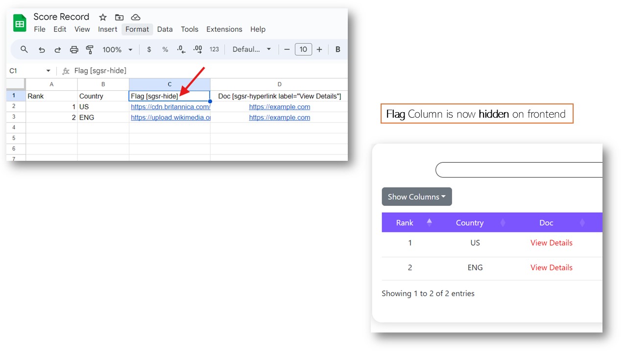
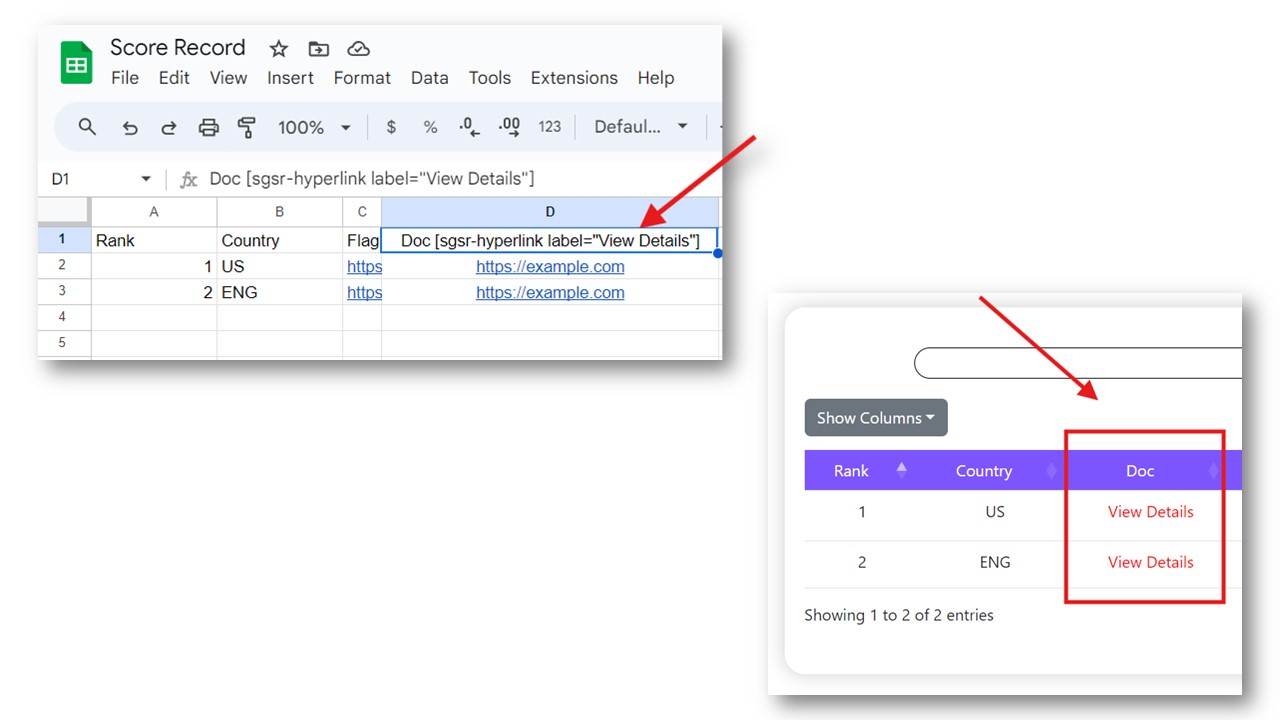
The [sgsr-hyperlink label="Click to view"] shortcode allows you to create a customizable hyperlink within your content. By specifying the label attribute, you can define the text that will appear as the clickable link.

Attribute	Description	Accepted Values	Example
label="Click to view"	Defines the text that will be displayed as the hyperlink.	Any text string.	label="More details"

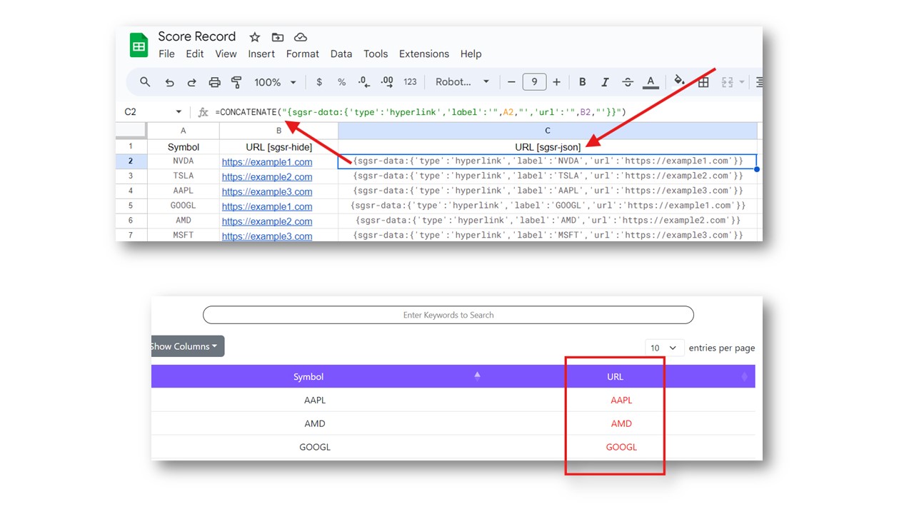
To create custom labels for each hyperlink using the [sgsr-json] code, you'll need to adjust your Google Sheets column header accordingly. For each cell where you want a hyperlink, format it using the following formula:

=CONCATENATE("{sgsr-data:{'type':'hyperlink','label':'",B2,"','url':'",D2,"'}}")

This formula combines the label from cell B2 and the URL from cell D2 into a JSON object, which can be processed by the [sgsr-json] code to generate a customized hyperlink.

Attribute	Description	Accepted Values	Example
type="hyperlink"	Specifies that the data is a hyperlink.	"hyperlink"	type="hyperlink"
B2	Defines that the label text will be taken from cell "B2".	Any cell reference.	B2, C2 etc.
D2	Defines that the URL will be taken from cell "D2".	Any cell reference.	B2, C2 etc.

See Live Examples

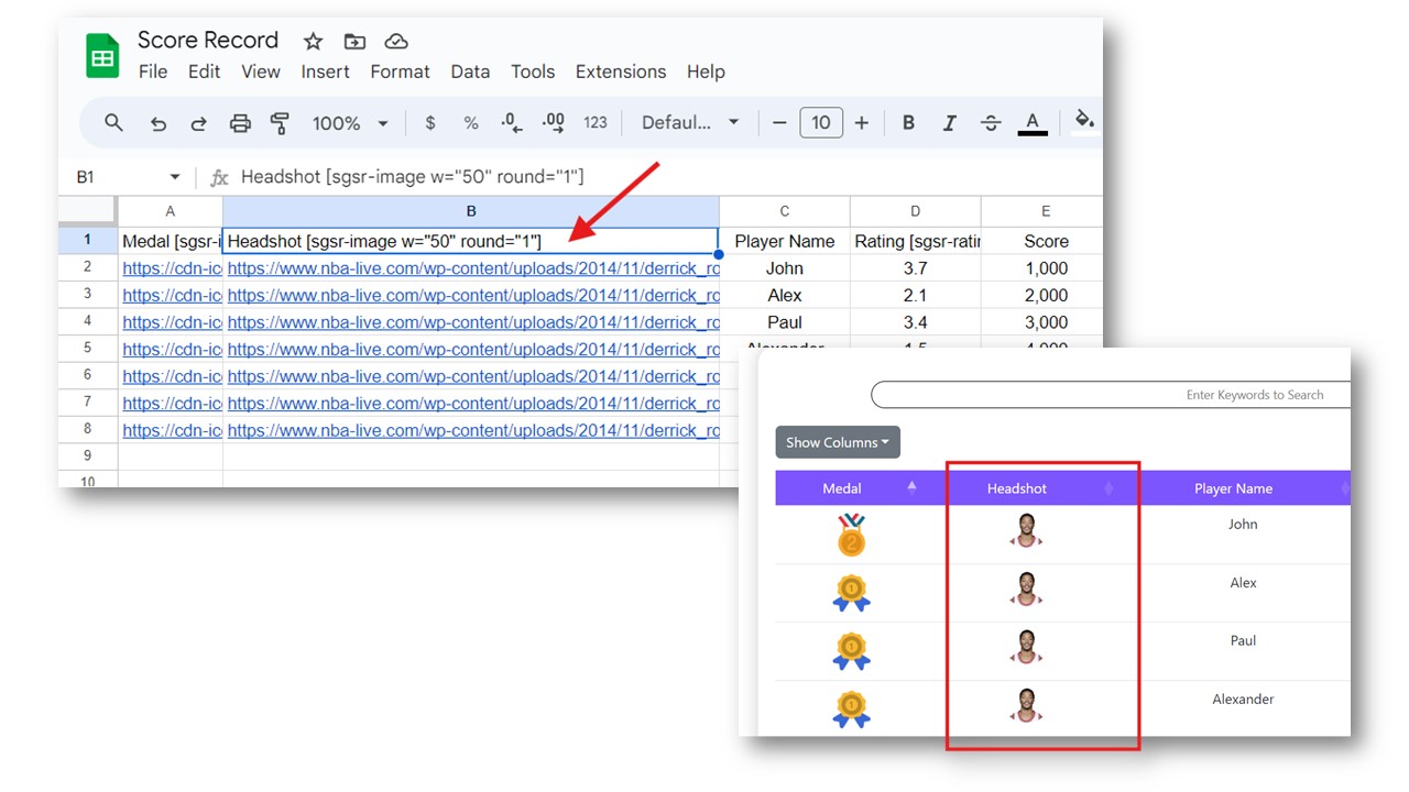
The [sgsr-image w="50" round="1"] shortcode allows you to display images directly within your content. By specifying the w and round attributes, you can control the size and shape of the image.

Attribute	Description	Accepted Values	Example
w="50"	Defines the width of the image in pixels.	Any positive integer value.	w="50"
round="1"	Determines whether the image should be round or square.	1 for round, 0 for square.	round="1"

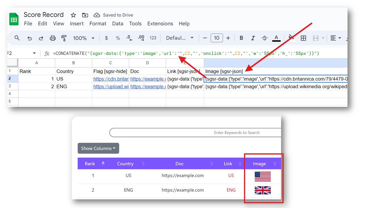
To further customize image embedding using the [sgsr-json] code, you can dynamically create image elements within your Google Sheets by using the following formula:

=CONCATENATE("{sgsr-data:{'type':'image','url':'",C2,"','onclick':'",C2,"','w':'55px','h':'55px'}}")

This formula combines the URL from cell C2 into a JSON object, which can be processed by the [sgsr-json] code to generate a customized image element.

Attribute	Description	Accepted Values	Example
type="image"	Specifies that the data is an image.	"image"	type="image"
C2	Defines that the image URL will be taken from cell "C2".	Any cell reference.	C2, D2 etc.
onclick (optional)	Specifies the URL to redirect to when the image is clicked.	Any valid URL or cell reference.	C2
w (optional)	Specifies the width of the image in pixels.	Any valid CSS width value.	w="55px"
h (optional)	Specifies the height of the image in pixels.	Any valid CSS height value.	h="55px"

See Live Examples

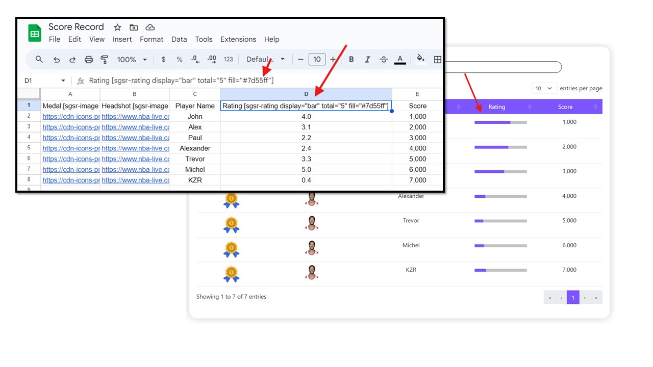
The [sgsr-rating display="star" total="5" fill=""] shortcode allows you to display rating values in your data table using customizable star or bar formats. By specifying the display, total, and fill attributes, you can control the appearance and scale of the rating.

Attribute	Description	Accepted Values	Example
display="star"	Defines the visual representation of the rating.	"star", "bar"	display="star"
total="5"	Sets the maximum value for the rating scale. If a rating higher than this value is entered, it will be converted into a weighted average out of this total.	Any positive integer value	total="100"
fill=""	Specifies the color of the stars or the bar, allowing you to customize the appearance to match your design preferences or branding.	Any valid color code (e.g., #ffcc00)	fill="#ffcc00"

You can place this shortcode in the header of a column in your Google Sheets to visually represent the ratings in your data table. The shortcode will automatically convert numerical ratings into the specified star or bar format based on the attributes you've defined.

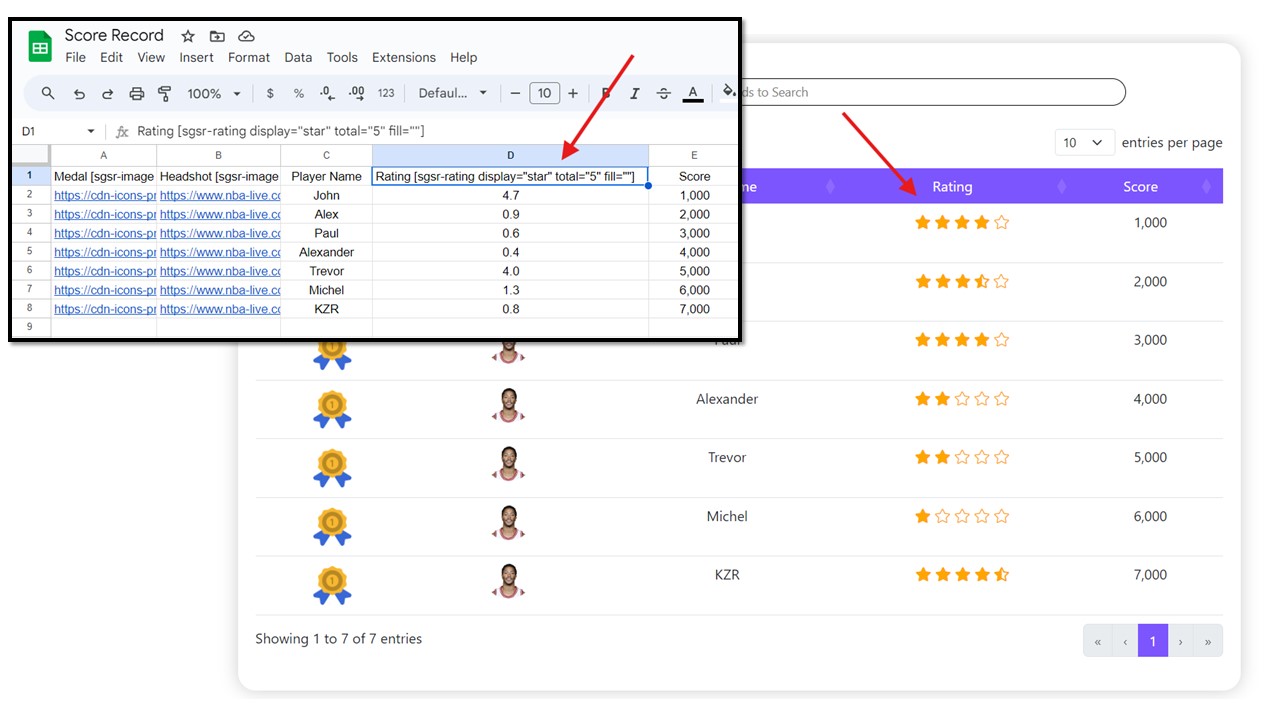
This shortcode is especially useful for displaying user ratings, scores, or any metrics that benefit from a visual representation. Whether you choose stars or bars, the `[sgsr-rating]` shortcode provides a flexible and aesthetically pleasing way to showcase your data.



See Live Examples

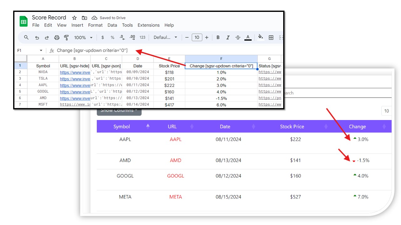
The [sgsr-updown criteria="0"] shortcode allows you to visually represent changes in values by displaying them with up or down arrows, based on a specified criterion. This is particularly useful for displaying stock price changes, performance metrics, or any data where a visual indicator of increase or decrease is needed.

Attribute	Description	Accepted Values	Example
criteria="0"	Defines the breakpoint between up and down values. If set to 0, negative values will be shown with a down arrow, and positive values with an up arrow. If set to another value, such as 10, values greater than 10 will be displayed with an up arrow, and those below 10 with a down arrow.	Any numerical value	criteria="0"

Dynamic Arrows: The shortcode dynamically assigns up or down arrows to values based on the criteria you define. This allows you to quickly and easily identify trends or changes in your data.

Custom Breakpoints: You can customize the threshold for what constitutes an "up" or "down" value. For example, setting criteria="10" would mean any value above 10 is shown with an up arrow, while any value below 10 is shown with a down arrow.

Example Usage:
Add this shortcode to the header of a column in your Google Sheets. The shortcode will then automatically apply the up or down arrows to the values in that column based on the specified criteria, making it easy to visualize changes at a glance.

See Live Examples

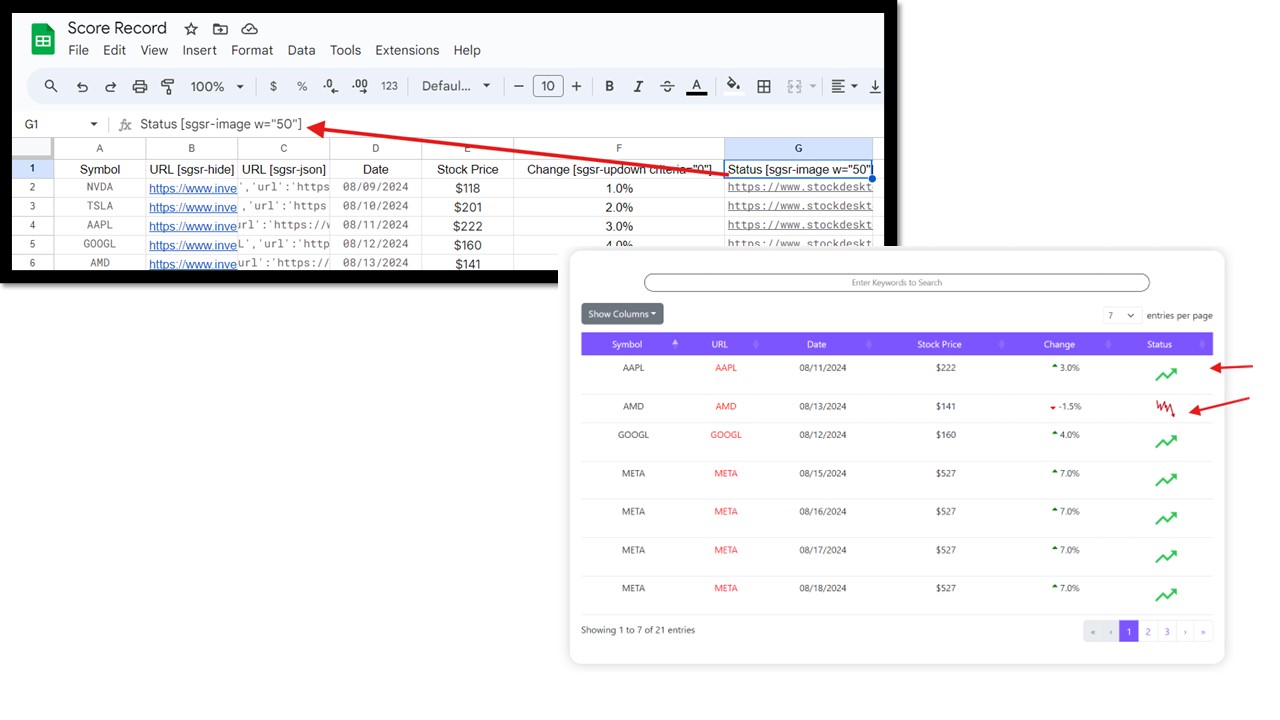
Showing trends with images:
The [sgsr-image] tag can also be used in the column header to display images. You can dynamically set if or else conditions to place URLs in the column based on the value in another cell. This allows you to show trend indicators, such as arrows, badges, or other symbols, that reflect changes or specific conditions in your data.

For example, you might display a green upward arrow image if a stock's price has increased, and a red downward arrow image if it has decreased, based on the values in another column. This dynamic approach helps in visually communicating data trends and statuses more effectively.

See Live Examples

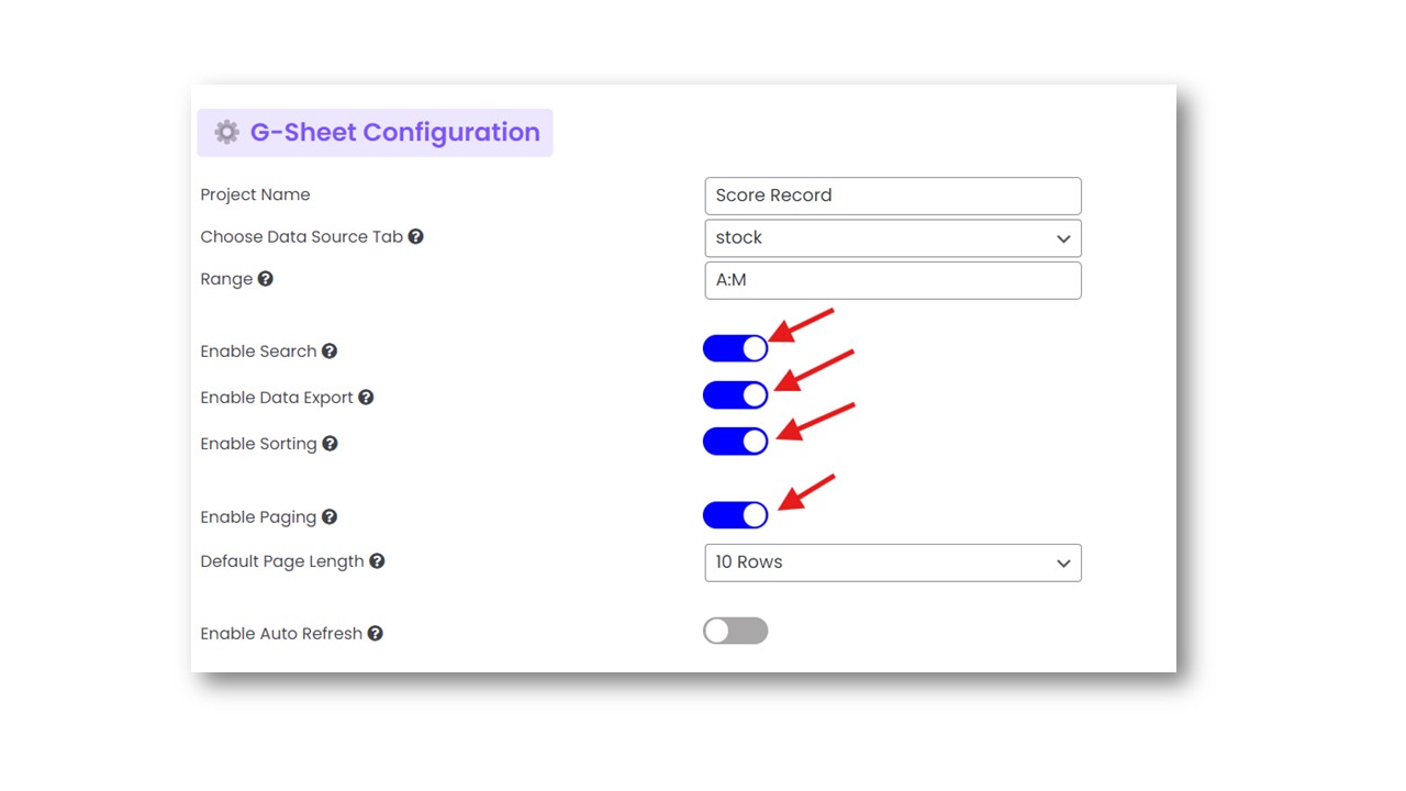
The sorting and search options in the admin menu are designed to provide robust functionality for managing and navigating large data sets with thousands of rows. These features ensure that even extensive tables can be easily managed and analyzed.

• Strong Search and Filter Functionality: The search option allows you to quickly locate specific data within large tables. The filter function can be used to refine search results further, making it easier to focus on relevant information without manually scanning through entire data sets.


• Pagination-Independent Sorting and Search: The sorting and search functionalities are fully integrated with the table’s pagination. This means that even when your data is split across multiple pages, the sorting and search operations will cover the entire data set, not just the currently visible page. This ensures that you can always find and sort data accurately, regardless of how the table is paginated.

These features combine to make the admin interface both powerful and user-friendly, particularly when working with large and complex data tables.

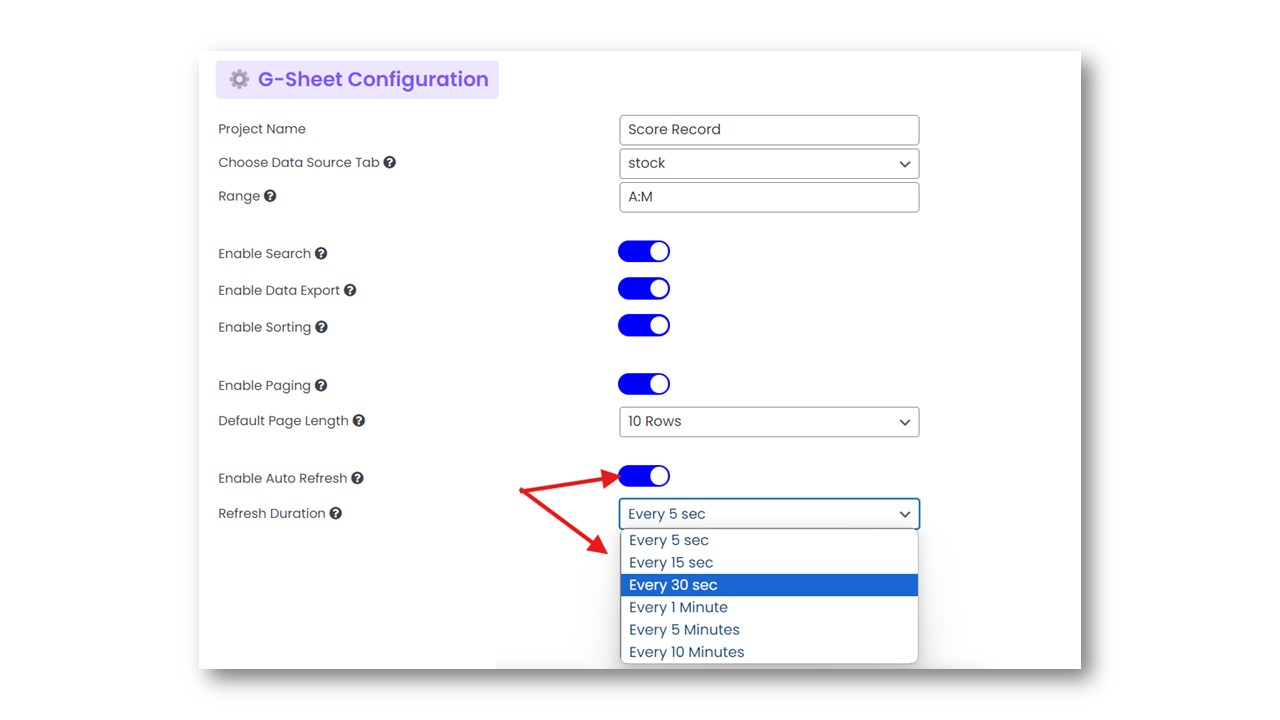
The auto-refresh feature in the admin menu updates your data tables in real-time without needing a page reload.

• Enable Auto Refresh: Activate this option to keep data current automatically, reflecting any changes instantly.


• Customizable Refresh Duration: Choose how often the table refreshes, from every 5 seconds to every 10 minutes, ensuring updates are as frequent as needed.

This feature ensures up-to-date data presentation, ideal for real-time monitoring, all without interrupting the user's experience.

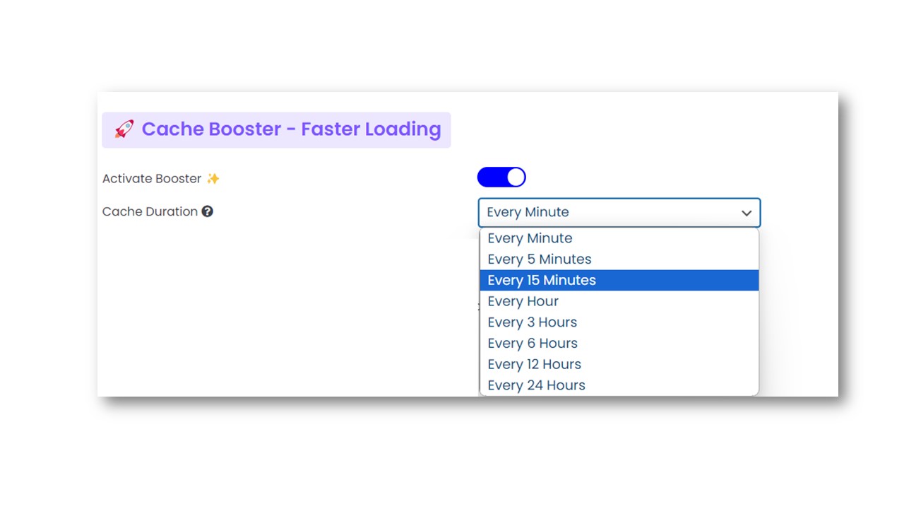
Activate caching to significantly boost your table's loading speed, especially if you're working with large datasets containing thousands of rows. This feature is particularly useful for data that updates infrequently, such as once a day, hourly, or every few minutes.

• Activate Booster: Enabling this option caches your data, allowing it to load faster by reducing the need to fetch updated data on every page load.


• Cache Duration: Choose the cache duration that best suits your data's update frequency, from every minute to every 24 hours, ensuring optimal performance while keeping your data up-to-date.

Enabling caching not only enhances loading speed but also helps conserve your daily usage limits (i.e., Hits), making it an efficient tool for managing resource usage, especially when dealing with large data tables.